08. 1D Gaussian
1D Gaussian
At the basis of the Kalman Filter is the Gaussian distribution, sometimes referred to as a bell curve or normal distribution. Recall the rover example - after executing one motion, the rover’s location was represented by a Gaussian. It’s exact location was not certain, but the level of uncertainty was bounded. It was unlikely that the rover would be more than a few meters away from its target location, and it would be nearly impossible for it to show up at the 50 meter mark.
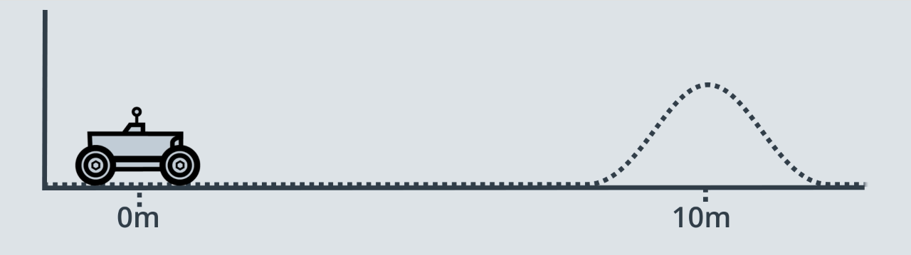
This is the role of a Kalman Filter - after a movement or a measurement update, it outputs a unimodal Gaussian distribution. This is its best guess at the true value of a parameter.
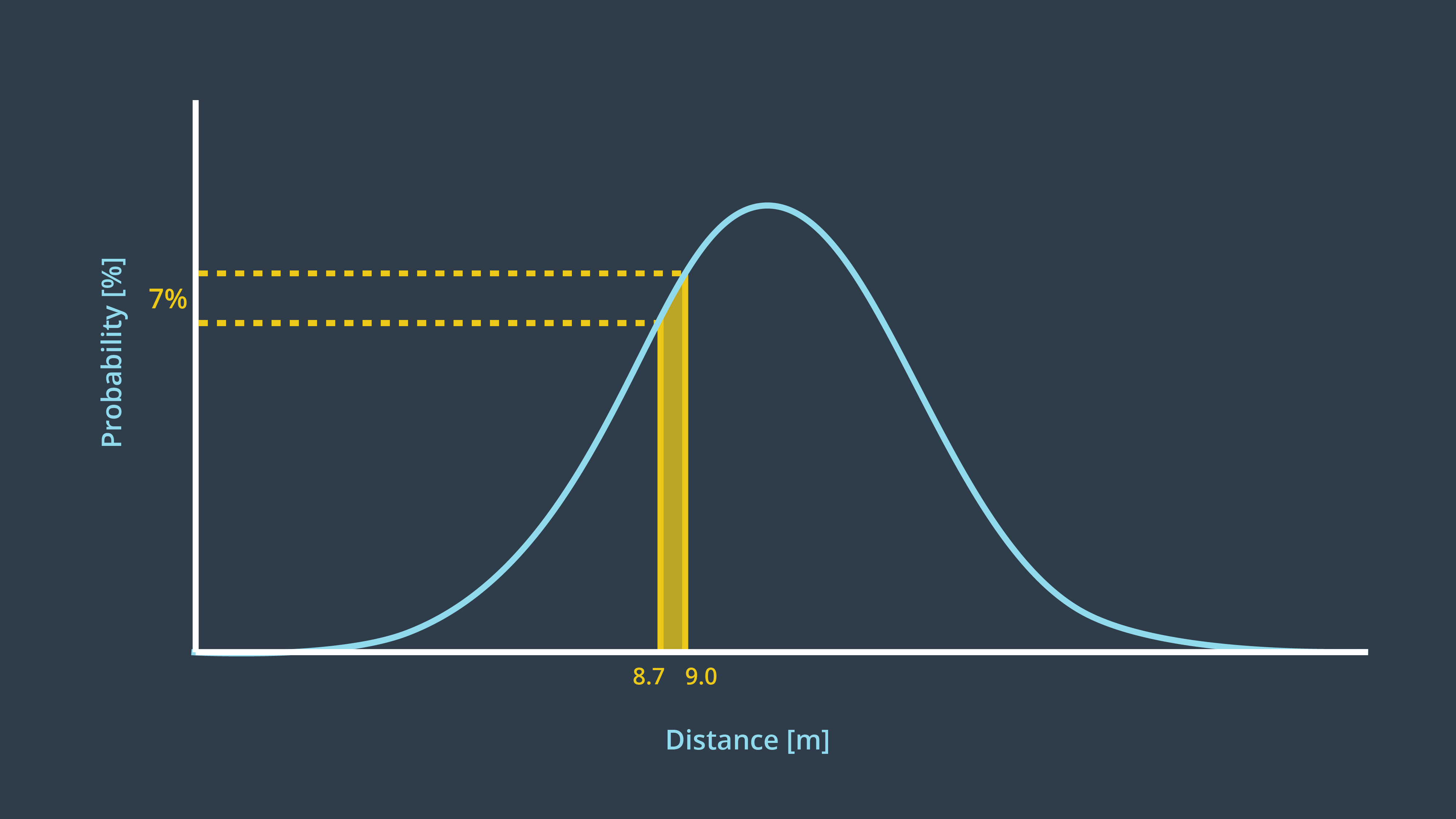
A Gaussian distribution is a probability distribution, which is a continuous function. The probability that a random variable, x, will take a value between x_1 and x_2 is given by the integral of the function from x_1 to x_2 .
In the image below, the probability of the rover being located between 8.7m and 9m is 7%.
Mean and Variance
A Gaussian is characterized by two parameters - its mean (μ) and its variance (σ²). The mean is the most probable occurrence and lies at the centre of the function, and the variance relates to the width of the curve. The term unimodal implies a single peak present in the distribution.
Gaussian distributions are frequently abbreviated as N(x: μ, σ²), and will be referred to in this way throughout the coming lessons.
It's time for a quiz! Reference the image below to answer the quiz question.
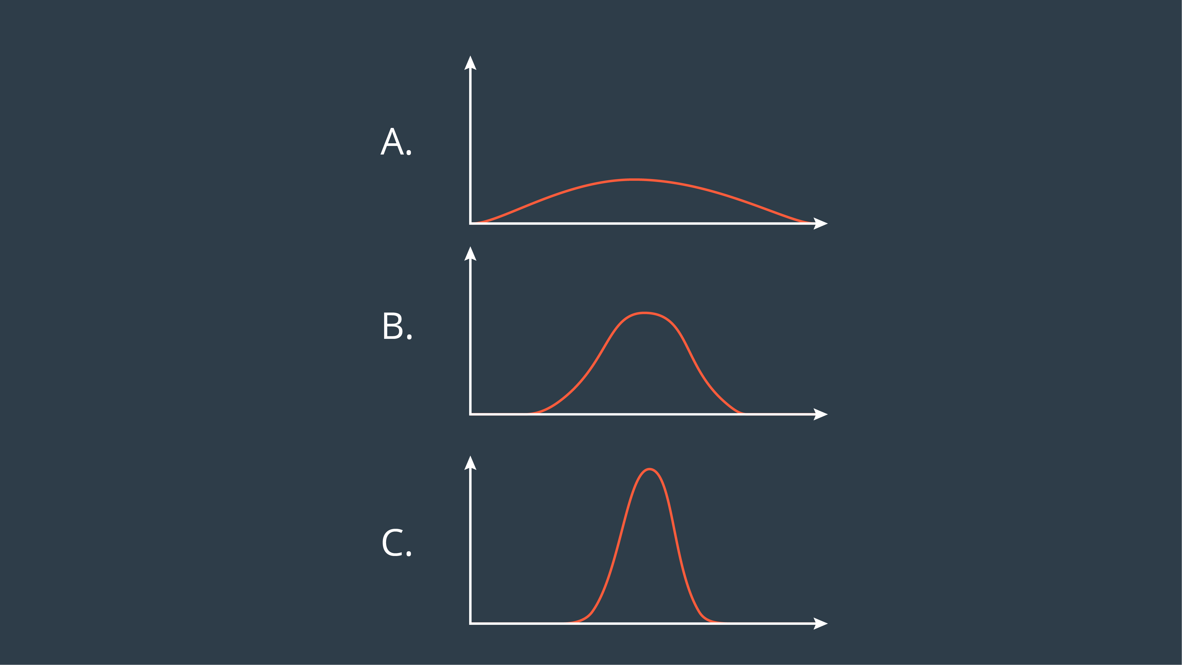
SOLUTION:
- C
The formula for the Gaussian distribution is printed below. Notice that the formula contains an exponential of a quadratic function. The quadratic compares the value of x to μ, and in the case that x=μ, the exponential is equal to 1 ( e^0 = 1 ). You’ll note here, that the constant in front of the exponential is a necessary normalizing factor.
Just like with discrete probability, like a coin toss, the probabilities of all the options must sum to one. Therefore, the area underneath the function always sums to one.
Now that you are familiar with the formula, it’s time to code the Gaussian in C++. This will allow you to calculate the probability of a value occurring given a mean and a variance!
Start Quiz:
Great, you’ve coded the formula for a Gaussian distribution, now let’s make sure you know where it is applied!
SOLUTION:
- Predicted Motion
- Sensor Measurement
- Estimated State of Robot
That’s right, the Kalman Filter treats all noise as unimodal Gaussian. In reality, that’s not the case. However, the algorithm is optimal if the noise is Gaussian. The term optimal expresses that the algorithm minimizes the mean square error of the estimated parameters.
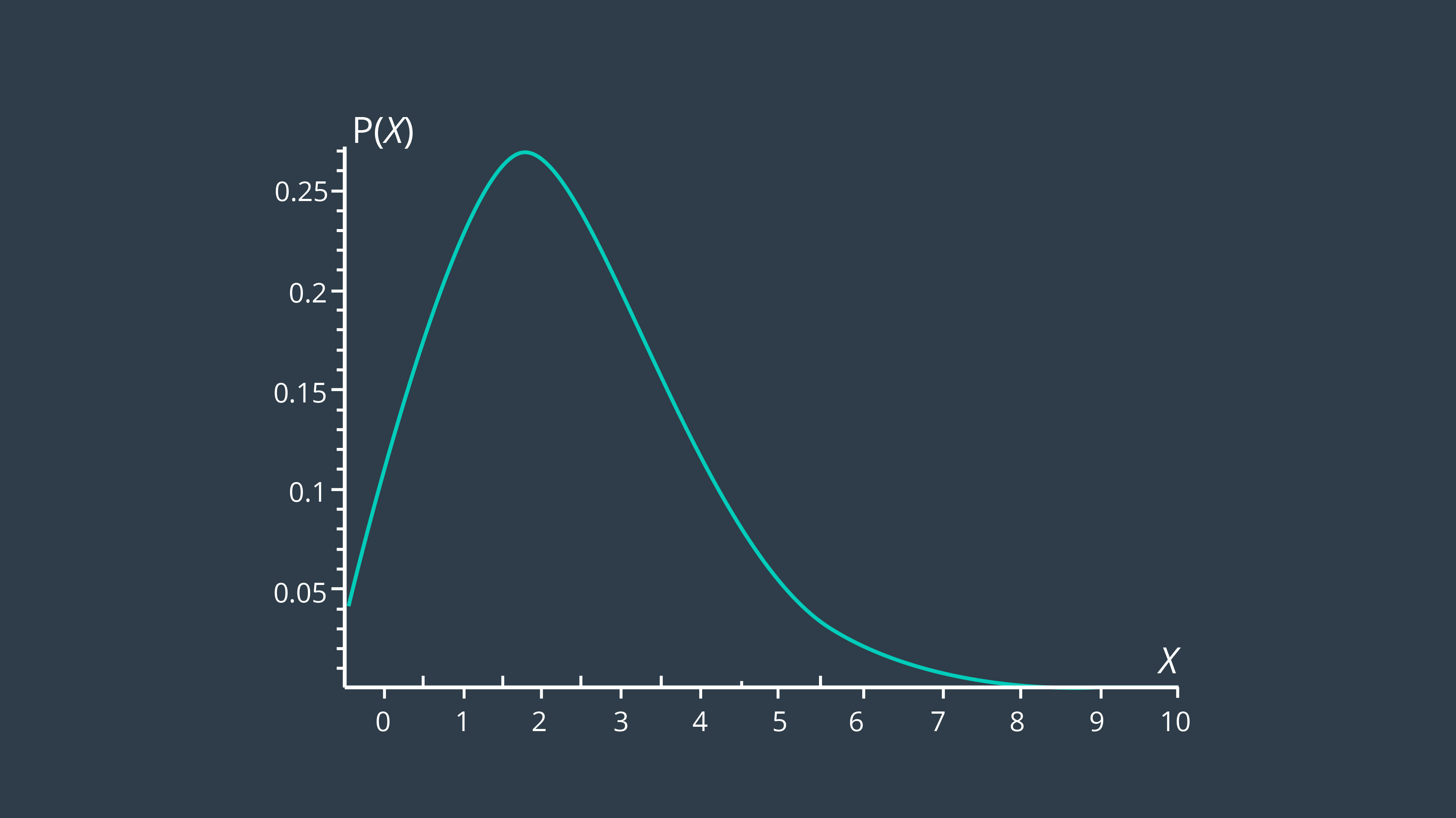
Distribution Quiz
Reference the following probability distribution to answer the quiz question below.
SOLUTION:
NoThat’s all of the mathematics that you need to know for now. Let’s start designing Kalman Filters!